Draw a plot by describing it. You name a table, a mark to draw (points, bars,
lines and so on), and which column goes to which part of the picture. That is
a specification, and gog draws it as an SVG.
One engine, written in Rust, does the drawing for R, Python, Julia and JavaScript. You write the specification in your language's own syntax, and the engine draws the same picture from it in all four, byte for byte.
One vocabulary instead of many chart types. There is no histogram()
function, so there are no arguments that belong to a histogram alone. The
whole vocabulary fits on one page, and each chart type is a combination of
words from it. A histogram is bar * bin: the bar mark joined to the bin transform,
which counts the rows in each interval. Keep bin and change bar to
line, area or step, and the same counts are drawn as a line, a filled
area or a staircase. You learn each word once, and it works the same way in
every plot.
It says no, and says what to write instead. If you write something the
grammar has no meaning for, gog refuses it, and the message says what to
write instead. It never accepts part of what you wrote and then ignores it, so
a plot that is drawn shows everything you wrote.
The same picture from four languages. A colleague who works in Python, Julia or JavaScript writes the same specification in that language's syntax, and gets the same file, byte for byte. So a team that uses different programming languages can still work on one plot.
A plot is a specification, not drawing code. What you build is a specification, and the engine draws it. So you can save one to a file, compare two of them, create one from another program, or send one over a network. That is harder in a library where a plot exists only as an object in your running session.
Things that usually need a second package are already here. Three dimensions, animation, brushing (selecting rows and dimming the rest), circular layouts, maps, networks, treemaps, flow diagrams and contour maps are all part of the same vocabulary. None of them is an add-on with a syntax of its own.
install.packages("gog", repos = c("https://psychometrician.r-universe.dev",
                                  "https://cloud.r-project.org"))
gog is not on CRAN yet. It is published on r-universe, so the
repos argument names r-universe first. The second address is CRAN, where R
finds the packages gog needs, such as jsonlite. On macOS and Windows,
r-universe builds a binary that includes the engine, so you do not need to
install Rust.
On Linux the same command installs from source and compiles the engine. That build needs Rust 1.75 or newer and a network connection. Install Rust first if the machine has none, or only an older version:
curl --proto '=https' --tlsv1.2 -sSf https://sh.rustup.rs | sh -s -- -y
source "$HOME/.cargo/env"
Compiling the engine can need more memory than a small machine has, such as a small Posit Cloud project. If memory runs out, the install stops and prints R code that downloads an engine that is already built.
If you want to change the engine rather than use it, build the package from a copy of the source repository. The book's R chapter shows how.
library(gog)

gm <- data.frame(
  gdp       = c(1000, 8000, 30000),
  life      = c(52, 68, 79),
  continent = c("Africa", "Asia", "Europe")
)

p <- data(gm) + point + x(gdp, scale = "log") + y(life) + color(continent)
save_svg(p, "life.svg")
Read that aloud: "Given gm: points, x is gdp on a log scale, y is life, color by continent." gog calls a line of code like this a sentence, and each part of it becomes one phrase of what you read aloud. So you can say a plot in words first, and then type it.
save_svg() writes an SVG, which stays sharp at any size. For a document or a
slide, save_png(p, "life.png") saves the same plot as a PNG picture of 1600
by 1200 pixels.
Every name you use from gog has a help page with an example that runs, such
as ?point or ?save_png.
When a plot does not draw as you expect, save_json(p, "plot.json") saves what
the engine reads to draw it: the sentence, and every value of each column the
sentence names. The engine draws the same plot from that file, so attach the
file to a bug report. Read it before you share it, because it holds your data.
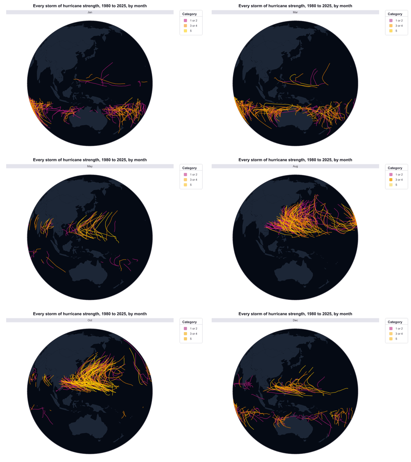
Each picture below was drawn from the code under it. Each example downloads
its table from the website of the book, gog's online manual, with
gog_table(). So the code runs without changes on a computer that is
online. Click a picture to open its page in the book, where you can turn the
3-D plots with the pointer.
The examples assume you have already run library(gog).
cyclones <- gog_table("cyclones")
cyclones$month <- factor(cyclones$month, levels = month.abb)
world_borders <- gog_table("world_borders")

p <- data(world_borders) + zone + x(lon) + y(lat) + group(country) +
  style(color = "#1c2636") +
  data(cyclones) + path + x(lon) + y(lat) + group(storm) + color(category) +
  palette(c("mediumvioletred", "darkorange", "gold")) + style(opacity = 0.6) +
  play(month) + globe(turn = 135, tilt = 10) +
  theme(background = "#050a14", grid = "none") +
  title("Every storm of hurricane strength, 1980 to 2025, by month")
save_gif(p, "hurricanes.gif")
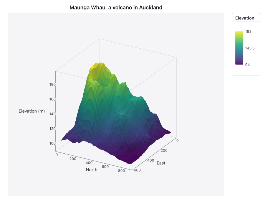
maunga_whau <- gog_table("maunga_whau")

p <- data(maunga_whau) + surface + x(east) + y(north) + z(elevation) +
  color(elevation) + palette("viridis") +
  z_label("Elevation (m)") + title("Maunga Whau, a volcano in Auckland")
save_svg(p, "volcano.svg")
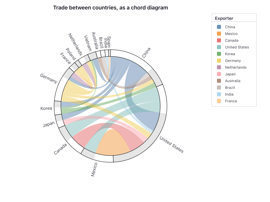
trade_partners <- gog_table("trade_partners")

p <- data(trade_partners) + x(billions) +
  ribbon * flow(exporter, importer, shared = TRUE) + color(exporter) +
  zone * flow(exporter, importer, shared = TRUE) +
  text * flow(exporter, importer, shared = TRUE) + label(name) +
  polar() + title("Trade between countries, as a chord diagram")
save_svg(p, "chord.svg")
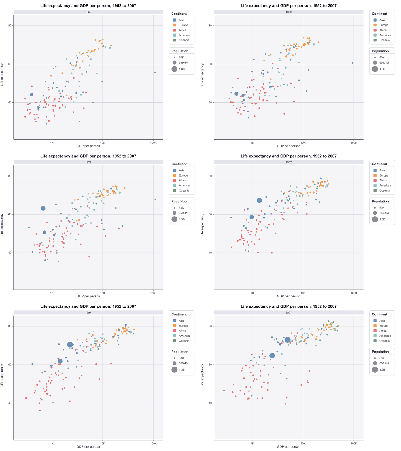
gm_all <- gog_table("gm_all")

p <- data(gm_all) + point + x(gdp, scale = "log") + y(life) +
  color(continent) + size(population) + play(year) +
  x_label("GDP per person") + y_label("Life expectancy") +
  title("Life expectancy and GDP per person, 1952 to 2007")
save_gif(p, "gapminder.gif")
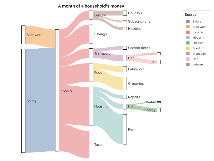
budget <- gog_table("budget")

p <- data(budget) + y(amount) +
  ribbon * flow(source, target, layered = TRUE) + color(source) +
  zone * flow(source, target, layered = TRUE) +
  text * flow(source, target, layered = TRUE) + label(name) +
  title("A month of a household's money")
save_svg(p, "sankey.svg")
Marks — points, lines, bars, areas, steps, error bars, boxes, ribbons, text, paths, reference lines, shaded regions, surfaces in three dimensions, and the links of a network.
Ways to show a column — position, color, size, shape, texture, transparency, a text label, or a split into one series per group.
Transforms, written into the sentence — binning, counting, shares, sums, averages, medians, quantiles, running totals, ranges, confidence intervals, smoothing curves, least-squares lines and density estimates, and the layouts of treemaps, flow diagrams, networks and cluster trees. The engine computes them, so you do not compute them before you plot.
Panels, spaces and animation — small multiples in rows or columns, several plots side by side or one above another, a circular (polar) space, a three-dimensional cube, maps and globes, and animation with one frame for each value of a column.
Selection — a brush selects the rows inside a range you give. Those rows keep their full color, and the other rows are dimmed. In a web browser you can also drag the brush with the pointer. On a flat plot, resting the pointer on a point, a bar or a text label shows the values of its row, with or without a brush. A mark that a transform moves or summarizes shows none.
Words and numbers — a title, a subtitle and a caption, a name for each axis, and three ways to write a number: as a percent, short with K, M, B or T, or with the number of decimal places you choose.
Chart types come from these words too: a pie chart is a stacked bar chart in polar space, and a violin plot is a density drawn as a ribbon.
The book is gog's full manual, free online. The engine draws every plot in it each time the book is built, so no picture in it is a screenshot.
https://psychometrician.github.io/gog-book/
The book shows its examples in R, Python, Julia and JavaScript. To run an
example that uses one of the book's tables, read the table first, for example
gapminder_2007 <- gog_table("gapminder_2007"). The book's
R chapter lists what is particular to R.
Apache License 2.0, declared in DESCRIPTION. The attribution notice,
inst/NOTICE, is installed
with the package. R itself includes the Apache license text, in
share/licenses, so this package does not include a second copy.